Machine
Learning (ML) and Artificial Intelligence (AI): ML Algorithms: Part- Eleven
by
Dr.
RGS Asthana
Senior
Member IEEE

Figure 1: Big Data, cloud technology
fuelling development of ML Algorithms [36]
Summary
ML
helps us create models, which can accurately answer what if questions about
certain things based on available data.
We
discuss in this paper the ML algorithms, such as, Linear
regression, Logical Regression, Clustering techniques like k-means & hierarchical,
decision tree, Neural networks. Naïve Bays classifier, support vector machines,
Backpropagation algorithm and deep learning methods.
Prerequisite
Read
article [1] to [16]
Keywords
Machine Learning (ML) Tools, Artificial Intelligence (AI), Neural Networks, Internet of Things (IoT), Data Science (DS), Deep
Mind, IBM’s Watson, K-means, Clustering
Prelude
Machine Learning (ML) is same as Machine Intelligence (MI). Human has
great capability of learning from experience. If we somehow inculcate this
capability of learning with experience in machines/computers then we have intelligence
in machines. ML
algorithms instruct computers in detail how to identify a cat in the photo; the
computer learns to do things on its own by using a suitable ML algorithm. The
experience in machines is, in fact, inculcated through training data.
Machines can
learn in three ways: viz. supervised
[S], semi-supervised learning (SS), unsupervised [U]and Reinforcement
[R] learning. In
S learning you need data with the ground truth i.e. one knows desired outcomes
for every data inputted, e.g. images are categorized into cats and dogs – the
algorithm finds out some features which help to distinguish data during
training. Then we show system or model unknown data and model has to make some
prediction. In SS learning, we know
outcome about a tiny subset of whole data only. This shows basically the very practical
situation. Further in U learning, data points have no
labels associated with them and goal of a U learning algorithm is to organize data
in some way or to identify and describe the underlying structure of data. R
learning is very close to SS. This can mean grouping it into clusters or
finding different ways of looking at complex data so that it appears simpler or
more organized. Reinforced
or R [29] learning algorithm chooses an action in response to each data point. The learning
algorithm also receives a reward signal a short time later, indicating quality
of the decision i.e. how good that decision was on correct or incorrect scale. Based on this algorithm employs a strategy
which yields the highest reward. R learning is the problem of getting an agent
to act in the world so as to maximize its rewards as shown in figure 2. Consider teaching a cat a new trick: you cannot
tell Cat what to do, but you can reward/punish Cat if it does the right/wrong
thing. It has to figure out what it did that made it get the reward/punishment,
which is known as the credit assignment problem. We can use a similar method to
train computers to do many tasks, such as playing backgammon or chess,
scheduling jobs, and controlling robot limbs.
R learning is also a natural fit for Internet of Things [16] applications. In
brief, an agent or even a human being can execute an action based on an
observation. It can repeat only that action where there is reward and not
penalty. S Learning implemented using Neural Net, can be thought of a problem
leading to memorization whereas R learning is a brute- force propagation of
outcomes to knowledge about states and actions or reasoning.

Figure 2: Reinforced learning – a powerful paradigm of AI
ML, AI, Mobile Technology, Big
Data, 3D Printing and Robotics are playing significant role (see figure 1).
What really marks healthcare different from other disciplines? Healthcare may often have very little labeled
data (e.g., clinical NLP). This may prompt the use of semi-supervised learning
algorithms i.e. keeping human in the loop (HITL). Sometimes, we have only small
numbers of samples (e.g., for a rare disease) and we need to learn as much as
possible from other data (e.g. EHR data of healthy patients). We may have lots
of missing data that too at varying time intervals and may only get censored
labels. Other more important problem which we need to solve is that ML base
algorithms do not give reason for arriving at a particular decision. Therefore,
it is pertinent to model the problem keeping these aspects in view and may be
reason for HITL in the solution.
ML
based solutions are good at prediction and diagnosis too is a prediction in a
way. We, therefore, describe ML based diagnosis and treatment systems. The only thing necessary for systems to give
better prediction is training on substantial data. The areas where ML/AI based
systems have impact in healthcare are: on-line consultations, Health
assistance and medication management, personal genetics, development of drugs of the
future, discovering new diseases, persistent care, discovering new clinical
pathways and last but not the least Robotics and Healthcare.
ML algorithms:
Linear
regression – The idea is to fit a line to the data points
so as to divide the points into two regions for this you can begin by moving
the line in arbitrary direction and minimize the error function which is
computed by adding distance from each point to line, least squares algorithm -
as we really don’t like negative numbers we use square of distance till we
minimize the error function which is addition of square of distance from each
point to line by doing number of hit and trials, Gradient descent – the aim is
to draw a line or curve to separate or split data, it can be done by giving
small penalties to points which are correctly found and giving big penalties to
points which are wrongly classified i.e. we make the error function continuous
and then we define probability function which should vary from 0 to 1. For
doing this, we define an activation function where 0 should map to 0.5 and huge
positive numbers map close to +1 and huge negative points map close to 0 which
is nothing but a Sigmoid function i. e. f(x) = 1/(1+e–x). We now try
to move the line till we reach a point where maximum number of points are
correctly classified i.e. we minimize the error function. We wish to make
product of probability in to addition and for doing this we take negative log
of the error function and this way we have our new error computation. In fact, predicting continuously is,
generally, referred to as a regression problem; an example could be autonomous
driving.
Logical Regression
- It is the go-to method for binary
classification or problems with two class values. We describe logistic regression algorithm
for ML.
The coefficients (Beta values b) of the logistic regression
algorithm must be estimated from your training data. This is done using
maximum-likelihood estimation.
The best coefficients would result in a model that would predict a
value very close to 1 (e.g. male) for the default class and a value very close
to 0 (e.g. female) for the other class. The intuition for maximum-likelihood
for logistic regression is that a search procedure seeks values for the
coefficients (Beta values) that minimize the error in the probabilities
predicted by the model to those in the data (e.g. probability of 1 if the data
is the primary class).
It is
enough to say that a minimization algorithm is used to optimize the best values
for the coefficients for your training data. When you are learning logistic,
you can implement it yourself from scratch using the much simpler gradient
descent algorithm.
Making predictions with a logistic regression model is as simple as
plugging in numbers into the logistic regression equation and calculating a
result.
Data preparation: It is a very important step before trying any type
of classification.
· Binary Output Variable: It predicts the probability of an instance
belonging to the default class, which can be mapped into a 0 or 1
classification.
· Remove Noise:
Logistic regression assumes no error in the output variable (y), consider
removing outliers and possibly misclassified instances from your training data.
· Gaussian distribution:
Logistic regression is a linear algorithm (with a non-linear transform on
output).
· Remove Correlated Inputs:
Like linear regression, the model can over fit if you have multiple
highly-correlated inputs. Consider calculating the pairwise correlations
between all inputs and removing highly correlated inputs.
·
Fail
to Converge: It is possible for the expected likelihood
estimation process that learns the coefficients to fail to converge.
Clustering [33] & [34]: It is a very important algorithm for unsupervised machine learning
and is a confirmed way to group the population or data points such that data
points with similar character are put in the same group or clusters. There are
mainly two types of clusters: in hard
cluster, each data point either belongs to a cluster or not. In Soft
Cluster, a probability or likelihood is associated with that data point
to a particular sector. Its applications include areas,
such as,
- Recommendation engines e.g. to suggest movies
one may like
- Market segmentation
- Social network analysis
- Search result grouping
- Medical imaging
- Image segmentation
- Behavioral segmentation:
1.
Segment
by purchase history
2.
Segment
by activities on application, website, or platform
3.
Define
personas based on interests
4.
Create
profiles based on activity monitoring
·
Inventory
categorization:
1.
Group
inventory by sales activity
2.
Group
inventory by manufacturing metrics
·
Sorting
sensor measurements
- Detect activity types in motion
sensors
- Group images
- Separate audio
·
Detecting
bots or anomalies:
1.
Separate
valid activity groups from bots
2. Group valid activity to clean up
outlier detection
K means clustering
K-means clustering
is a type of unsupervised learning and is generally used when the resulting
categories or groups in the data are unknown. X
K means is an
iterative clustering algorithm. It attempts to discover local maxima in every repeat
cycle see steps given below:
Steps
1: Choose the desired number of clusters K;
2: Allocate randomly each data point to a cluster;
3: Compute cluster centroids;
4: Re-assign each point to the closest cluster centroid;
5: Re-compute cluster centroids Now, re-computing the centroids
for both the clusters; and
6: Repeat
steps 4 and 5 until no improvements are seen.
Hierarchical clustering (or
Linkage Clustering), forms hierarchy of clusters. It
starts with each point being a separate cluster, and works by joining two
closest clusters in each step until everything is in one big cluster.
We can easily choose the number of clusters afterwards by cutting the tree
diagram horizontally where we find suitable. It is also repeatable but is of a
higher complexity (quadratic).
If data are not labeled, S learning is
not possible, and an U learning approach is required, which attempts to find
natural clustering
of the data to groups, and then map new data to these formed groups. The clustering
algorithm which provides an improvement to the support vector machines is
called support vector clustering and is often used in industrial applications either
when data are not labeled or when only some data are labeled as a preprocessing
for a classification pass.

Figure 3: Decision tree (Image taken from
Wikipedia)
Decision
tree - A decision
tree for a plane crash is drawn with its root at the top. Figure 3 shows the bold text
representing a condition or internal node,
based on which the tree splits into branches also referred to as edges.
The end of the branch that doesn’t split anymore is the decision or called leaf,
in this case, whether the passenger died or survived, represented as red and
green text respectively.
Neural networks [30]
- If we are unable to define a line to separate points into two categories we
may either use higher order function or multiple lines to define a region or a
plane. In such scenarios neural net have a role. A hidden layer in neural Net
only means that it neither an input nor an output layer

Figure 4: Linearly separable data
Two
classes can be linearly separable iff they can be separated by linear
combination of attributes, i.e., 1-D threshold, 2-D lines, 3-D Plane or a
hyper-plane (see figure 4).
Kernel trick is a way of
computing the dot product of two vectors x and y in some other feature space and to reduce overall computation. Kernel trick is interesting because the need to compute the
mapping may never arise If our algorithm can be expressed only as inner product between
two vectors, all we need is replace this inner product with the inner product
from some other suitable space. That is where the “trick” resides: wherever a
dot product is used, it is replaced with a Kernel function.
The kernel function denotes
an inner product in feature space and is usually denoted as: K(x, y) =
<φ(x), φ(y)>. Using the Kernel function,
the algorithm may be carried into a higher-dimension space without explicitly
mapping the input points into this space. This is highly desirable, as
sometimes our higher-dimensional feature space could even be
infinite-dimensional and thus unfeasible to compute.
Kernel functions
[32] are sometimes called "generalized dot product" also. ML algorithms model problems in an attempt to
solve a problem efficiently, e.g., we can map 2D data to 3D space by performing
a non-linear transformation say dot product, i.e., k(x,y) = f (x. W) and avoid
using a curve or a complex decision boundary and instead use a hyper-plane as
depicted in figure 5 & 6. Tanh is another popular activation function with
range -1 to +1 i.e. it is zero centered. Both Sigmoid and tanh functions suffer
from vanishing gradient problem. RELU function easy on computation as compared
to Sigmoid and tanh activation function.
The RELU function is invariably used today for the hidden layers and
output layer still uses Sigmoid or Tanh function.

Figure 5: Sigmoid function S (z) =
1/ (1+e−z)
which is non-linear in nature, monotonically increasing and is also continuously
differentiable

Figure
6: Rectified Linear Units Function R(x) (the step
function is similar to R(x)) is defined below:

Naïve Bays classifier [35]
It’s good to know about
Bayes theorem which works on conditional probability. It tells that something will
happen, given that something else has already occurred. Using the
conditional probability, we can calculate the probability of an event using its
prior knowledge.
Below is the formula for calculating the conditional probability.
Where
- P (H)
is the probability of hypothesis H is found to be true. This is known as
the prior probability.
- P (E)
is the probability of the evidence
- P (E|H)
is the probability of the evidence if hypothesis is true.
- P (H|E) is the probability of
hypothesis if evidence is found.
Naive
Bayes classifier uses the Bayes Theorem and predicts membership probabilities
for each class such as the probability that given record or data point belongs
to a particular class. This is also known as Maximum A-posteriori Probability (MAP). The MAP for a
hypothesis is:
MAP(H)=max(P(H|E))=max((P(E|H)*P(H))/P(E))=max(P(E|H)*P
(H))
Where P (E) is evidence probability, and is used only
to normalize the result.
Naive Bayes classifier assumes that all co-relation
among the features is zero. Presence or absence of a feature does not influence
the presence or absence of any other feature.
As an
example we consider three classes associated with
Animal Types say, Parrot,
Dog and Fish. We also consider four predictor features as
Swim, Wings, Green Color and Dangerous Teeth.
It can
be said that for Parrots: 10% parrots can swim, all parrots have
wings, 80% parrots are Green and 0% parrots have Dangerous Teeth according to data provided.
As
per data for Dogs, 90% dogs can swim, 0% dogs have wings, 0% dogs are of Green
color and 100% dogs have Dangerous Teeth.
Data
for fishes show that 100% can swim, 0% have wings, 20% fishes are of Green
color and only 10% fish have Dangerous Teeth.
We will demonstrate the Naive Bayes approach using
above example.
For Hypothesis testing for the animal to be a Dog:
P
(Dog | Swim, Green, Teeth) = P (Swim |Dog) * P (Green |Dog) * P (Teeth |Dog) *
P (Dog) / P (Swim, Green, Teeth)
= 0.9 * 0 * 1 * 0.333 / P (Swim, Green, Teeth) = 0
= 0.9 * 0 * 1 * 0.333 / P (Swim, Green, Teeth) = 0
For
Hypothesis testing for the animal to be a Parrot:
P
(Parrot| Swim, Green, Teeth) = P (Swim |Parrot) * P (Green |Parrot)* P (Teeth| Parrot)
* P (Parrot) / P (Swim, Green, Teeth)
= 0.1 * 0.80 * 0 *0.333 / P (Swim, Green, Teeth) = 0
= 0.1 * 0.80 * 0 *0.333 / P (Swim, Green, Teeth) = 0
For
Hypothesis testing for the animal to be a Fish:
P
(Fish |Swim, Green, Teeth) = P (Swim |Fish) * P (Green |Fish) * P (Teeth |Fish)
*P (Fish) / P (Swim, Green, Teeth)
= 1 * 0.2 * 0.1 * 0.333 / P (Swim, Green, Teeth) = 0.00666 / P (Swim, Green, Teeth)
= 1 * 0.2 * 0.1 * 0.333 / P (Swim, Green, Teeth) = 0.00666 / P (Swim, Green, Teeth)
The
denominator of all the above calculations is same i.e. P (Swim, Green, Teeth).
The value of P (Fish | Swim, Green, Teeth) is the only positive value
greater than 0. Using Naive Bayes, we can predict that the class of this record
is Fish.
As computed value of probabilities is very low, we use P
(Swim, Green, Teeth) only to normalize these values.
Support Vector Machines (SVM) - It is binary classification [36] S ML algorithm. Each data item is plotted as a point in n-dimensional space
(where n denotes # of features). Then, classification is carried out by finding
the hyper-plane that distinguishes the two classes [37]. Support Vectors are the co-ordinates of individual
observation. Support Vector Machine chooses the best (maximum margin) hyper
plane (see figure 7) not only farthest to the nearest point but also separates
the two classes hyper-plane/ line.

Figure 7: Maximum-margin hyperplane and margins
for an SVM trained with samples from two classes. Samples on the margin are
called the support vectors [37, 40].
Large Margin Decision Boundary [40]: The separator has
to be as far as possible. This means that we have to maximize the margin. We
can normalize the equation of the separator so the distance in the supports are
1 or −1, by r = (wTx + b)/||w||. So the length of the optimal margin
is m = 2/||w|| {see figure 6}. This means that maximizing the margin is the
same that minimizing the norm of the weights.
Calculating the decision Boundary: Given a set of
examples {x1, x2,... , xn} with class labels yi
∈ {+1, −1} The decision
boundary that classify the examples correctly holds yi(wTxi
+ b) ≥ 1, ∀i. This redefines the problem of
learning the weights as an optimization problem (see [40] for details).
Solving XOR through a Neural Net
The XOR (see figure 8) network opened
the door to far more interesting neural network and ML designs. An implementation Of XOR function using
logical gates is shown in figure 7 and a network version is shown in figure 10.

Figure 8: XOR problem [39]
Truth Table
Input
output
A B
X
0 0 0
0 1 1
1 0 1
1 1 0
Figure 9
shows the four points as shown in the truth table and no single linear function
can separate the red and blue points.
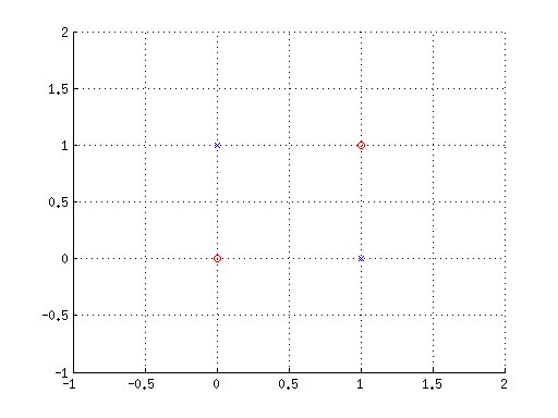
It is obvious that points are not
linearly separable. We
can also use Rectified Linear Units Function R (x) {see figure 5} instead of Sigmoid.

Figure 10: Implementation of XOR function using
Neural net with one hidden layer. ‘h1’ gives output of a logical ‘OR’ function;
‘h2’ reverses the input or is flip side of logical ‘OR’. In other words, ‘h1’
and ‘h2’ correspond to one hyper-plane each. Sigma is, in fact, a sigmoid
function and ‘b’, ‘b1’ and ‘b2’ is bias for output and hidden layer element ‘h1’
and ‘h2’ respectively.
Output of element h1(figure 9) Output of element h2 Final output X
Sigma(20*0+20*0-10)=0 Sigma(-20*0-20*0+30)=1 Sigma(20*0+20*1-30)=0 Sigma(20*1+20*1-10)=1 Sigma(-20*1-20*1+30)=0 Sigma(20*1+20*0-30)=0 Sigma(20*0+20*1-10)=1 Sigma(-20*0-20*1+30)=1 Sigma(20*1+20*1-30)=1 Sigma(20*1+20*0-10)=1 Sigma(-20*1-20*0+30)=1 Sigma(20*1+20*1-30)=1
Output ‘X’ corresponds to XOR
function (see truth table).
Backpropagation
in ANN
The backpropagation
algorithm trains a given feed-forward multilayer neural network for a given set
of input patterns with known classifications. When each entry of the sample data
set is presented to the network, the network examines its output response to
the sample input pattern. The training is done using an S learning method and the error function
is computed using the ANN's output and a known expected output given in the
data set. Error function is presented to
the ANN and it is used to modify its internal state. In fact, the backpropagation
algorithm is a way for computing the weights [44].
Following steps are
part of any Backpropagation algorithm:
Initialize
Network: Each
neuron (also called Unit in ANN) has a set of weights that needs to be
maintained. One weight for each input connection and an additional weight for
the bias. We generally initialize the
network weights to small random numbers say, in the range of 0 to 1.
Forward Propagate: We can compute an output from an ANN by propagating an input signal
through each layer until the output layer outputs the desired values. This is
referred to as forward-propagation. We
can calculate an output from ANN by propagating an input signal through each
layer until the output layer outputs its values. We call this forward-propagation which has three
distinct parts:
Neuron Activation - The input could be a row from our training
dataset, as in the case of the hidden layer. It may also be the outputs from
each neuron in the hidden layer, in the case of the output layer. Neuron
activation is calculated as the weighted sum of the inputs like linear
regression layer by layer
hj =
∑ wij * xi + bj where h is jth hidden layer,
w is weight and b is bias for the layer
i
We then apply the activation function and repeat the same for the
next layer. This part is broken down into two sections:
Neuron Transfer - Once a neuron is activated, we need to transfer
the activation to see what the neuron output actually is.
Transfer functions used may be the sigmoid
activation function (see figure 4). Recently, the rectified Linear Units transfer function (see
figure 5) has become popular, particularly, with deep
learning networks.
Forward
Propagation - Forward propagation is implemented for a row of
data from our dataset with ANN.
Back Propagate
Error: Error is computed using the expected outputs
given in data and the actual outputs forward propagated from the ANN. This
involves multiple iterations of exposing a training dataset to the network back-propagating
the error and then modifying the network weights.
The error is then computed and propagated
backward through the ANN from the output layer to the hidden layers.
Transfer Derivative – We need to remember and may use three steps of
calculus before we go forward:
1.
Derivative: it is d/dx xn= H x n-1
i.e. if equation of a curve is y=x2
Then its derivative F(x) = 2 x.
2.
Partial derivative (Example) f(x, y) = y3 +
3 x*y then ðf/ ðx=3y and
ðf/ ðy= 3y2 + 3x i.e. we treat all other variables as
constant.
3.
Chain rule:
Problem if f(x) = 2x and g(x) = x2 then f (g(x)) = 2x2
Chain rule: d/dx [f (g (x))] = f’ (g (x))*g’ (x)
Solution: So f (g(x)) = 2x*2
= 4x
Given an output value from a unit, we need to compute slope. The
network is trained using gradient descent.
The first step is to calculate the error for each output neuron; this
will give us our error signal (input) to propagate backwards through ANN.
Update Weights – We need to move opposite to the derivative. Once errors are calculated for each unit in
the network via the back-propagation method layer by layer, they can be used to
modify the ANN unit weights.

The equation above shows the gradient
descent update rule, where ‘W’ is weight, learning rate ‘α’ pronounced as Alpha (amount in
percentage by which ANN unit weight can change in every iteration) - a parameter we are required to give, J is error and is computed by the back-propagation procedure for units of
ANN and input is
the input value that caused the error (see Figure 11). Back-propagation of errors is used to optimize and update
weights during gradient descent. Please note that back-propagation is a
recursive process.
A few words on the learning rate, because it is one of the
important hyper-parameters (“settings” for ANN) that one has control over. Too
high learning rate can force that one does not get to the minimum one is
searching for as one mat jump over it. Similarly if learning rate is set very low, ANN may
take long time to get to the right weights, or may get stuck in a local
minimum. It may be a good idea to arrive at the right value of learning rate by
trying several values for it and pick the value that works the best for your ANN
and dataset. A neural net or ANN could be
a massive composite function and chain rule may be used to reduce computation. A similar method is used for
the bias weight, except that either there is no input term, or input is the
fixed value of 1.0.

Figure 11: Weight Reduction
process; if we repeat the
process enough, one finds oneself nearly at the bottom of the curve and
much closer to the optimal weight configuration for ANN [45]. We need to use a
differentiable function to find its derivative, i.e. a non-linear function.
Remember that the input for the output layer is a collection of
outputs from the hidden layer. Now
we know how to update network weights, we need to figure out how to do it
repeatedly.
Training Network: As is
stated before, ANN is modified using stochastic gradient descent. This involves first looping for a fixed
number of periods and within each period updating the network for each row in
the training dataset. Because updates are made for each training pattern, this
type of learning is called on-line learning. If errors were accumulated across
a period before modifying the weights, this is called batch learning or batch
gradient descent.

Figure 12: A MLP with two hidden layers is S learning network. Each time data is
processed by a layer; it gets multiplied by interconnection weights, then
summed and processed by a nonlinear activation function then sent to the
next layer. Finally the data is processed one last time within the output
layer to produce the neural network output [39]. Here y is the output unit and
x1, x2, … , xn are the inputs.
Predict: Making predictions with a trained neural network is easy
enough. We know how to forward-propagate an input pattern to get an output.
This is all we need to do to make a prediction. Figure 12 shows a MLP with bias. In fact an
ANN can be trained to realize any non-linear function.
Deep learning [31] - The term ‘Deep learning’ is derived from “deep”
neural nets built by layering many networks on top of each other [13].
Due to the increasing power and falling price of computer servers and advent of
cloud computing, machines with enough processing power are now available as
well as are capable to run such networks. Now you don’t need to own
infra but due to democratization of data you only pay for actual use by minute
as server- less environment is becoming common way of processing data today.
Deep learning models typically use back-propagation with
gradient descent. In ML, this feed forward architecture is known as the multilayer perceptron.
The difference between the ANN [2] and perceptron is that ANN uses a non-linear
activation function such as sigmoid as shown in figure 4 but the perceptron uses the step function (latest is ReLU which
is a non-linear function) and
this non-linearity gives the ANN its great control.
ANNs [2] are very
flexible yet powerful deep learning models and can model any complex function. If
our projected data belongs to a higher dimensional space then by carrying out a
non-linear transformation the data becomes linearly separable. The green hyper-plane
is the new decision boundary as shown in figure 13. This is equivalent to
drawing a complex decision boundary in the original input space (see figure 14).

Figure 13: Separation boundary is
plane
Further, the deepness of the network
is said to be directly proportional to number of hidden layers in the
network.
There are two areas viz., military and
healthcare where we have got to AGI level [13]. USA in Iraq and Afghanistan war
has used stealth aircrafts and drones which had human–in–the-loop (HITL)
capability only for ‘kill’ command but technology did not even need this. ML algorithms are very good at analyzing images
even better than human being, particularly, as it can process thousands of
images per second. It is used for this reason for identifying even very small
tumors from images. A doctor is used for finally selecting the images but it is
also not necessary. HITL
is required till neural net weights are set i.e. only during training phase but
use of HITL becomes voluntary after that.

Figure 14: complex Decision
boundary required to separate points
The
convolution neural nets are less useful if the data cannot be made to look like
an image as these nets only capture local spatial patterns.
It needs
no initial learning material as long as some feedback
mechanism is established to collect data while the system is
running.
In,
Reinforcement
learning a computer is able to assign a value to each right or wrong turn that
a rat might make on its way out of its maze. Each value is stored and all these values are updated as system learns.
Limitations of
reinforced learning: It is often too memory expensive
to store values of each state as the problems can be pretty complex. Solution to these problems led researchers to
look into areas such as Decision
Trees or Neural Networks to make this process practically computationally expensive.
In recent years, deep learning concept (see figure 2) is used to locate and recognize
patterns in data, whether the data refers to the turns in a maze, the positions
on a Go board, or the pixels shown on the screen and a suitable reward or
penalty is given for each move.
A
number of industrial-robot makers use this approach for training their robots
to perform new tasks without manual programming. Reinforcement learning is used
by Alphabet to make its data centers more energy efficient as a
reinforcement-learning algorithm can learn from data and suggest, say, how and
when to operate the cooling systems to save energy.
The
power of this software’s remarkably humanlike behavior is in self-driving cars.
The specific algorithm is needed for highway merging software and
it was demoed in Barcelona by Mobileye - an Israeli automotive company - that
makes vehicle safety systems used by dozens of carmakers including BMW. Google and Uber say they are also testing
reinforcement learning for their self-driving vehicles.
Way forward
There will be effort and progress
towards achieving AGI and ASI levels. This in turn means development of S ML,
i.e. without HITL. We will see more of AI based systems playing against AI [13]
and achieving new breakthroughs particularly in healthcare industry where there
are problems which human wish to solve; however, in other areas human are
likely to be more careful because of unknown risk factors.
A good example of system without HITL is
Cyber-knife [38] like solution developed in first decade of 21 century. It is a
non-invasive treatment. The CyberKnife system enables radiation oncologists to
deliver high doses of radiation with pinpoint accuracy to a broad range of
tumors to any part of the body. The patient may be treated of tumor say within
a week. The
GammaKnife [41] is treatment for adults and children with small to medium brain tumor, a nerve condition that
causes chronic pain, and other neurological conditions. In 2007, UCSF acquired the Perfexion Leksell Gamma \Knife
[42], which offers extreme accuracy, efficiency and
outstanding therapeutic response.
CyberKnife as well as GammaKnife technologies are used to
treat both cancerous and non-cancerous tumors [43], but GammaKnife is limited
to only treatment above the ear and in the cervical spine. However, CyberKnife
is dedicated Robotic System for SRS and stereotactic body radiotherapy (SBRT),
capable of treating cancer throughout the entire body. GammaKnife
is in use since 1950s however CyberKnife provides equivalent results for
certain tumors and a better outcome for others. Further, CyberKnife is FDA
cleared since 2001 for treatment of tumors throughout the entire body. Both these technologies are strong
candidates for AI (with or
without HITL) to give hopefully a better performance.
References
[1]
Progress and Perils of Artificial Intelligence (AI) http://newblogrgs10.blogspot.in/2017/04/progress-and-perils-of-artificial_5.html
[2] Invited Chapter 6 - Evolutionary Algorithms and Neural
Networks, Pages
111-136, R.G.S. Asthana in book, Soft Computing and Intelligent
Systems (Theory and Applications), Academic Press Series in Engineering,
Edited by:Naresh K. Sinha, Madan M. Gupta and Lotfi A. Zadeh ISBN:
978-0-12-646490-0
[3] Future 2030 by
Dr. RGS Asthana, Senior Member IEEE
[4] Machine Learning
(ML) and Artificial Intelligence (AI) – Part 1, by Dr. RGS Asthana, Senior Member IEEE
[5] Machine Learning
(ML) and Artificial Intelligence (AI) – Part Two, by Dr. RGS Asthana, Senior
Member IEEE
[6] Machine Learning
(ML) and Artificial Intelligence (AI): Cognitive Services and Robotics – Part
Three by Dr. RGS Asthana, Senior Member IEEE
[7] Machine
Learning (ML) and Artificial Intelligence (AI): Big Data and 3 D Printing
– Part four by Dr. RGS Asthana, Senior Member, IEEE.
[8] Machine Learning
(ML) and Artificial Intelligence (AI): Drones and Self-driving Cars– Part
Five by, Dr. RGS Asthana, Senior Member IEEE
[9] Machine Learning
(ML) and Artificial Intelligence (AI): Healthcare– Part Six by, Dr. RGS
Asthana, Senior Member IEEE
[10]
Machine Learning (ML) and Artificial Intelligence (AI):
Will AI/ML intelligence surpass humans? Part Seven by Dr. RGS
Asthana, Senior Member IEEE
[11] Machine Learning
(ML) and Artificial Intelligence (AI): Impact of AI/ML
in Healthcare: Part-Eight by Dr. RGS Asthana, Senior Member IEEE
[12] Machine Learning
(ML) and Artificial Intelligence (AI): Big data &
Data Science (DS) and their importance: Part-Nine by Dr. RGS Asthana, Senior Member IEEE
[13] Machine Learning (ML) and
Artificial Intelligence (AI): Super-Intelligence - Are
we afraid?: Part-ten; by Dr. RGS Asthana, Senior Member IEEE.
[14] Deep mind
website
[15 IBM Watson
Website
[16] Internet of Things (IoT)
[17] How to use ML in Mobile
[19] Product recommendation versus Product discovery
[20] Our
product categorization just took a quantum leap with AI and Machine Learning
[21] How
can e-commerce retailers leverage predictive analytics to make smarter, quicker
decisions about marketing strategy?
[22] Fraud detection and prevention
[23] Is the future of ecommerce is predictive analytics?
[24] How to use ML in mobile applications? P?
[25] Phone apps driven by Artificial Intelligence
[26] Niki Web-site
[27] ios based apple app store - itunes
[28] Google play website
[29] Friendly Introduction to Machine Learning
[30]
Neural Networks
[31] Applied Deep Learning - Part 1: Artificial Neural Networks
[32] Kernel Functions for Machine Learning
Applications
[33] An Introduction to Clustering and different methods of clustering
[34] Clustering Algorithms: From Start to State Of The Art
[35] How the Naive Bayes classifier works in
ML
[36]
The 10
Algorithms Machine Learning Engineers Need to Know
[37] Understanding Support Vector Machine algorithm from examples
(along with code)
[38] Website: Cyber-knife
[39]
Introduction: The XOR Problem
[40] 06 svm.pdf
[41] UCSF Medical Centre: Gamma Knife
Thank you for your blog.Really looking forward to read more.
ReplyDeleteMySql Admin training
MYSQL online training
MYSQL training
OBIEE online training
OBIEE training
Oracle 11g rac online training
Oracle 11g rac training
Oracle Access Manager online training